Yt μt γt εt t 1 T. A representation thof the dynamics of an N order system as a first order differential equation in an N-vector which is called the state.

State Space Representations Of Linear Physical Systems
Non-standard Matlab commands used in this tutorial are highlighted in green.
. Define State-space Model A 0 1 -1 -3 B 1 0 C 1 0 D 2 ssmodel controlssA B C D H controlss2tfssmodel printH Step response for the system t y controlstep_responseH pltplott y plttitleStep Response H pltxlabelt pltylabely pltgrid pltshow 0 0 1 1 3 0 1 0 1 0 0 2 State-space Model. Poles of a closed-loop system can be found from the characteristic equation. Ft is a p m matrices.
This technique can be used for linear or nonlinear time-variant or time-invariant systems. In this chapter let us discuss how to obtain transfer function from the state space model. To dealing with multivariable state-space model is most convenient.
Recall from the State-Space Tutorial page we can use a pole placement technique to obtain the desired output. U r - Kx r - Kv control input. Y t μ t γ t ε t t 1 T 11 where μt.
An AR1 model FollowingHamilton1994b 373374 we can write the first-order autoregressive AR1 model y t y t 1 t as a state-space model with the observation equation y t u t and the state equation u t u t 1 t where the unobserved state is u t y t. If the entire state space for a problem is given then it is possible to trace the path from the initial to goal state and identify the sequence of operation required for doing it. Y t 1 0 α t α t 1 ϕ 1 ϕ 2 1 0 α t 1 0 η t.
We know the state space model of a Linear Time-Invariant LTI system is - dotXAXBU YCXDU Apply Laplace Transform on both sides of the state equation. Where all the distributions are Gaussian. Gt is a p p matrices.
AR MA and ARMA models in state-space form See SS Chapter 6 which emphasizes tting state-space models to data via the Kalman lter. State space models 3. Z t Z 1 0 and.
In this part a tool to setup the state-space model based predictive controller is provided. U u y Cx D x Ax B 1 This represents the basic state-space equation where x a vector of the first-order state variables y the output vector x. It describes a system with a set of first-order differential or difference equations using inputs outputs and state variables.
State-Space Models Overview 1. Create analyze and use state-space representations for control design. State-space models Linear ltering The observed data fX tgis the output of a linear lter driven by white noise X.
The setup program returns a function handle for the online MPC controller. The determinant of the sI-. State space model.
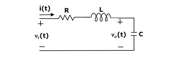
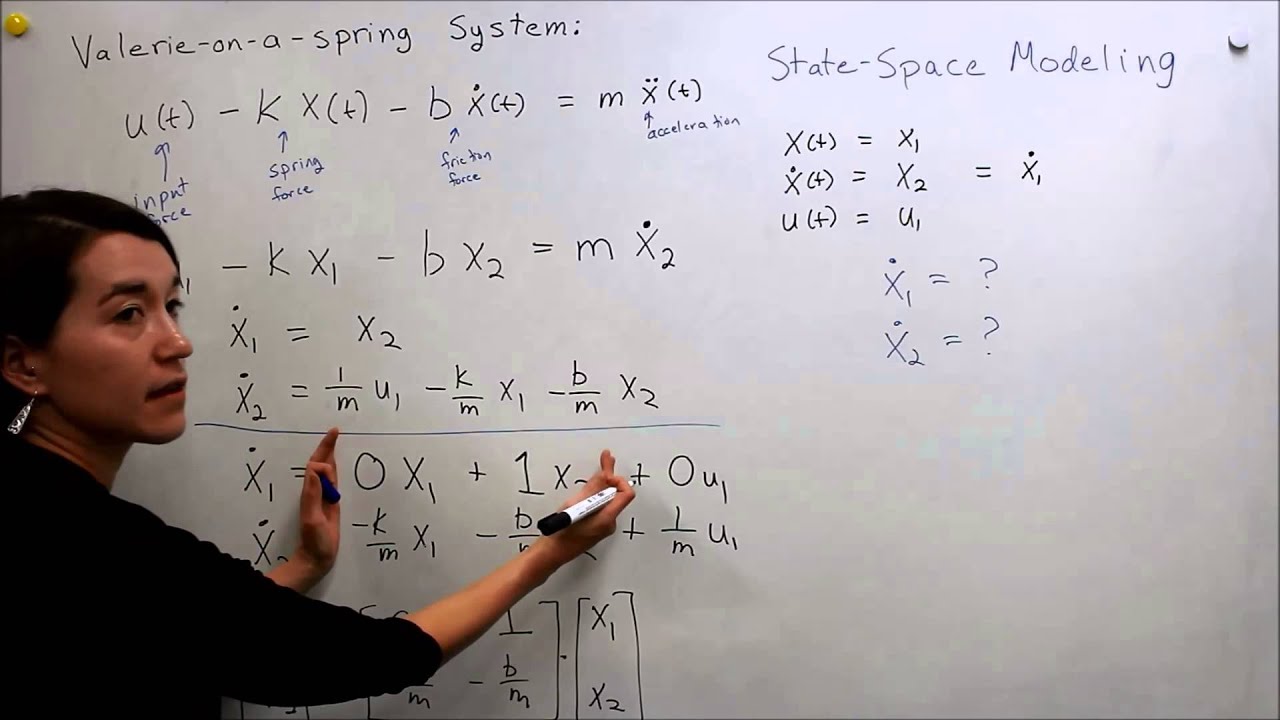
Second order mass-spring system. Key Matlab commands used in this tutorial. Wt yt xt NmFt xt.
This model is a workhorse that carries a powerful theory of prediction. A time series is a set of observations y1 yn y 1 y n ordered in time that may be expressed in additive form. A state-space model is commonly used for representing a linear time-invariant LTI system.
This lecture introduces the linear state space dynamic system. Advantages of State Space Search. 1 The local level model.
State-space equations Control design using pole placement Introducing the reference input Observer design. 1 An Intuitive Example of a State Space Model. State-Space Modelling by Kevin Kotzé.
For a SISO LTI system the state-space form is given below. The equation inside the State-Space block is. C0 xt xt 1 NpGt xt 1.
This is contained in the file T4-llmR. The process by which the state of a system is determined is called state variable analysis. It is easier to apply where Laplace transform cannot be applied.
ARIMA and RegARMA models and dlm 5. The first and the second equations are known as state equation and output equation respectively. Basic system model using the State-Space block.
Dynamical Linear Models can be regarded as a special case of the state space model. This tutorial will introduce the attendees to the analysis and forecasting of time series by state space methods using R. There are several different ways to describe a system of linear differential equations.
The linear state space system is a generalization of the scalar AR1 process we studied before. Matlab commands from the control system toolbox are highlighted in red. State space model tutorial In control engineering a state-space representation is a mathematical model of a physical system as a set of input output and state variables related by first-order State-Space Models 1 14384 Time Series Analysis Fall 2007 Professor Anna Mikusheva Paul Schrimpf scribe Novemeber 15 2007 revised November 24 2009.
Y C X D U. K state-feedback gain matrix. The first program for this session makes use of a local level model that is applied to the measure of the South African GDP deflator.
Once again the first thing that we do is clear all variables from the current environment and. State space models provide a very flexible framework that has proved highly successful in analysing data arising in a wide array of disciplines such as to mention a few economics business and finance engineering physics hydrology and. T t T ϕ 1 ϕ 2 1 0 R t R 1 0 η t ϵ t 1 N 0 σ 2 There are three unknown parameters in this model.
The state-space representation was introduced in the Introduction. This video is the first in a series on MIMO control and wil. It is very useful in AI because of it provides a set of all possible states operations and goals.
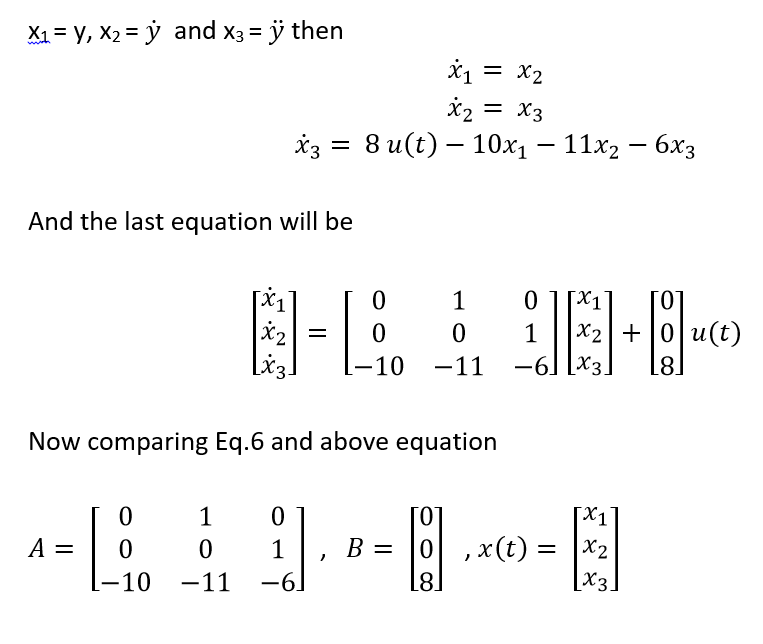
Advantages of State Space Techniques. Acker lsim place plot rscale. 1 2 where is an n by 1 vector representing the systems state variables is a scalar representing the input and is a scalar.
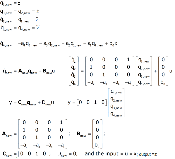
At this point the model is very general and an equation of any order can be set up for solution in the block parameters. Multivariable and State Space MPC V20. Representing dynamics of higher-order linear systems.
U and Y are input vector and output vector respectively. ARMA models in state space form AR2 model y t 1y t 1 2y t 2 e t e t NID0 2 Let x t y t y t 1 and w t e t 0. MPC Tutorial II.
In the absence of these equations a model of a desired order or number of states can be. This can be put into state space form in the following way. State-space models aka dynamic linear models DLM 2.
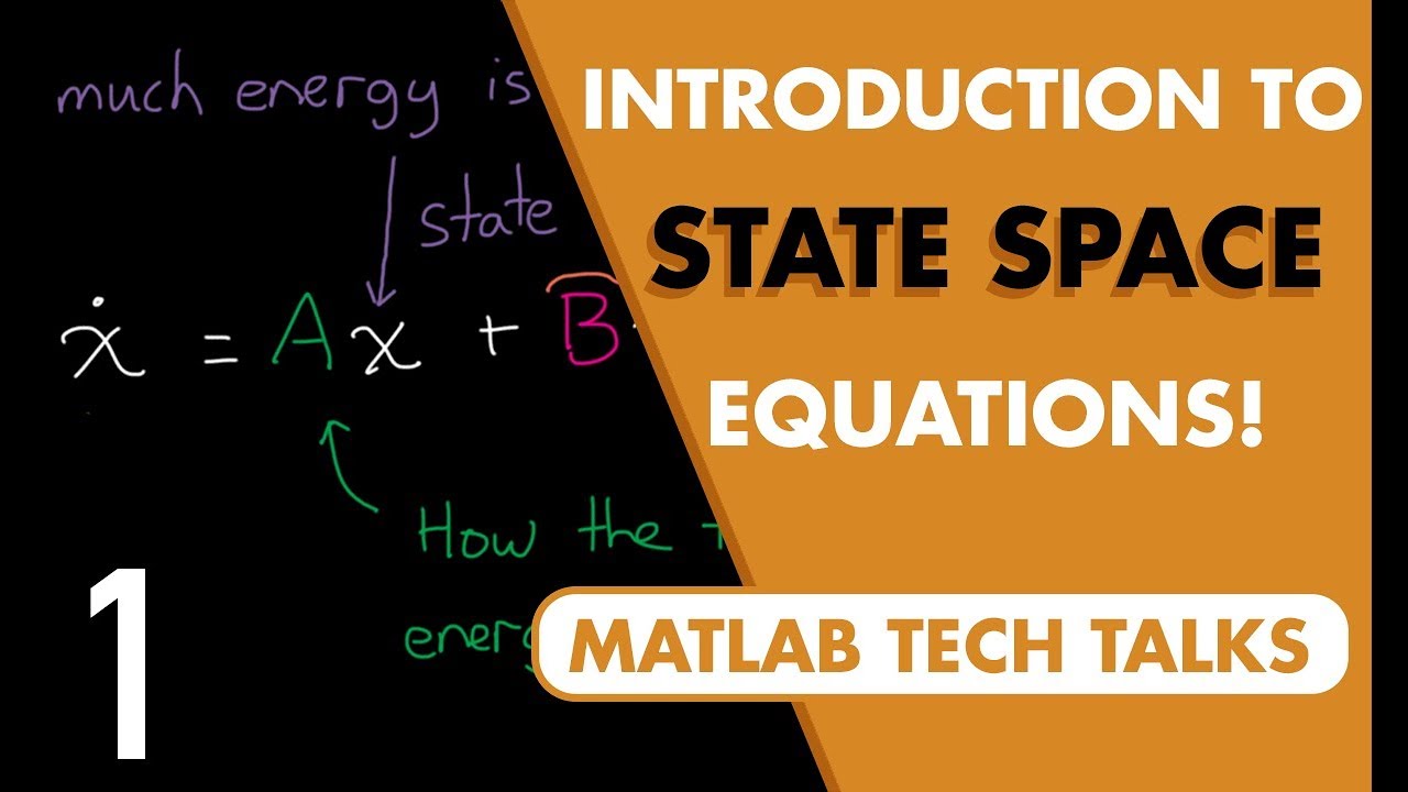
Lets introduce the state-space equations the model representation of choice for modern control. Sspace State-space models 7 Some stationary state-space models Example 1. ϕ 1 ϕ 2 σ 2.
Its many applications include. The state space model of Linear Time-Invariant LTI system can be represented as X A X B U. Then y t 1 0x t x t 1 2 1 0 x t 1 w t Now in state space form We can use Kalman filter to compute likelihood and forecasts.
Where X and X are the state vector and the differential state vector respectively. Transfer Function from State Space Model. Vt is a m m varianceco-variance matrix.
As planned this is the second part of the MPC series. Convert the Nth order differential equation that governs the dy namics into N first-order differential equations Classic example.
Control System State Space Model Javatpoint

State Space Analysis Of Control System Electrical4u
Control Systems State Space Model
State Space Representations Of Linear Physical Systems
Intro To Control 6 1 State Space Model Basics Youtube
State Space Part 1 Introduction To State Space Equations Youtube

State Space 11 Tutorial And Worked Examples Youtube

State Space Representations Of Linear Physical Systems
0 comments
Post a Comment